Look up a list of items and return matches in Google Sheets

Anyone who’s spent time in spreadsheets dreads receiving that request to match a random list of things with another of list of things. Right? Except when you are used to using VLOOKUP. That tried-and-true method is very good at finding a match in a list against a another (usually longer) list.

But what happens when you need to do multiple VLOOKUP-like requests at the same time, say when you have a list of Student IDs and need to look up a list of corresponding names?

Wouldn’t it be great if you could do that in only a single step instead of multiple columns, tabs, and a long process?

Luckily, there’s a trick you can use in Google Sheets to take those multiple lookups and turn them into a single formula.

TL;dr – Matching each item in a list against another list

Why does this matter, anyway?

Looking up a list one item at a time is slow. Looking up all of the terms in a list is really useful, especially when you have a long list of IDs and a long list of values that might or might not match that list. Also, this method works for comma-delimited lists of different lengths in adjacent rows (e.g. cell 1 listing attendance for course 1 has two students, and cell 2 listing attendance for course 2 has five students, and only two of the students overlap both courses.)

WHAT	WHY
Look up a list of ID values in Google Sheets, returning a new comma-delimited string with the results of your lookup	Transform a list in a single step

Recipe for building our formula

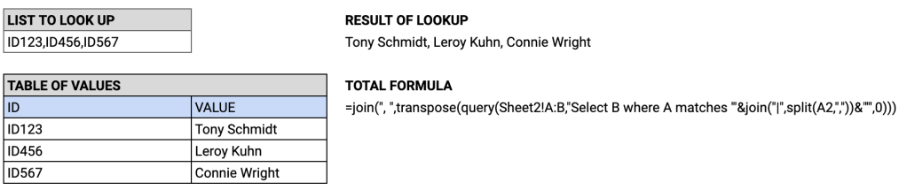
Given a comma delimited list of items you want to look up where the mapped value is not obvious, e.g. “ID123,ID456,ID567”, look each item up against a table of other information about that item where the lookup key is each item in the first list.

For example, you might have a list of Unique IDs and want to find out and return the corresponding mapped value, e.g. the name of people in a class. To do this you need to take the peopleID and return a name.

Each item in the list is the key you want to lookup in another list. One way to do this in multiple steps is to use VLOOKUP where you would run a vlookup to get a different value, e.g. to find that ID123 has the student name “Tony Schmidt”.

To do this lookup, you need to use the QUERY function in Google sheets to match multiple simultaneous conditions.

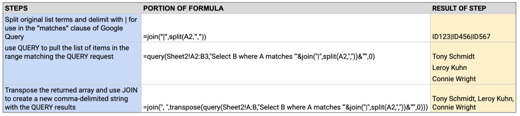
Using the matches keyword in QUERY, transform your comma-delimited list into a pipe-delimited list, then transpose and join the result to get a returned comma-delimited string from your QUERY function.

(fun fact: the QUERY function returns an Array which makes this possible.)

How does the formula work?

First, get the list items from our original list into a format that QUERY understands. The QUERY function in Google Sheets uses the term “matches” to look up one or more terms in the QUERY action. Using the the SPLIT function, we find each item in the comma-delimited list and then JOIN to replace commas with a “|” character, indicating item 1 OR item 2 so that the QUERY uses multiple terms to match.

After transforming our original list into a pipe-delimited list, we write a QUERY against the list we’re trying to match.

The goal is to select a term from column A (the one in the list with the keys matching our original list) with the corresponding value we want from column B (the ID value for each list item).

What does it look like when you’re done?

When finished, we took the original list of ID123, ID456, ID457 and turned into the keys (names) that matched these ids in our lookup table:

• ID123 matches “Tony Schmidt”
• ID456 matches “Leroy Kuhn”
• ID567 matches “Connie Wright”

Concatenating these and returning them yields the result “Tony Schmidt, Leroy Kuhn, Connie Wright.” If you wanted to make this fancier, you could use a string e.g.

="STUDENT NAMES:" & CHAR(10) & join(", ",transpose(query(Sheet1!A2:B3,"Select B where A matches '"&join("|",split(A2,","))&"'",0)))

To format your string further:

STUDENT NAMES:
Tony Schmidt, Leroy Kuhn, Connie Wright

Using the “&” to concatenate a string and the CHAR function to add a line break.

Now that you’ve seen the steps, go ahead and copy this original sheet to try it yourself. Happy Matching!